AIMMD toy tutorial: 1D double-well path sampling

This notebook is a self-contained tutorial that runs AIMMD on a cheap toy model: a single particle evolving on a 1D double-well free-energy surface (embedded in an MDAnalysis trajectory).

You will learn how to:

• define a toy engine (toy_mdrun) and metastable states (states_function),

• build an initial path and a minimal committor network,

• configure aimmd.Params and launch an AIMMD run,

• inspect the produced path ensemble and compute simple projections/free-energy estimates,

• (optional) switch to RFPS and run a small multistate example.

The notebook is written to be readable first; performance is irrelevant for this toy model. However, to obtain the expected results for this model, you may need to increase the runtimes to produce more sampling and / or training data, as the defaults are for illustration but may be insufficient to adequately sample this system.

You will need a working AIMMD installation. Although we do not use this functionality here, gromacs is required in your path, since - as an integral component of AIMMD - its availability is checked at import time. (Hint: if you are using conda environments and have a modules-based gromacs install, consider adding an activation hook that sources a gromacs module, as a bash file under path-to-env/etc/conda/activate.d/load_modules.sh)

0. Imports and working directory

The toy data folders will be created relative to the notebook location:

• ../data/1d_double_well/ for the double-well example,

• ../data/1d_periodic/ for the optional multistate periodic example.

If you want a clean restart, remove thoes folders manually.

import os
from math import inf
from pathlib import PosixPath

import aimmd
import MDAnalysis as mda
import matplotlib.pyplot as plt
import numpy as np
import torch
from scipy.special import expit

# Use the toy double-well folder shipped with the tutorial data.
DATA_DIR = PosixPath("../data/1d_double_well").resolve()
DATA_DIR.mkdir(parents=True, exist_ok=True)
os.chdir(DATA_DIR)

print("Working directory:", os.getcwd())

Working directory: /home/covino-shared/data/lichtinger/LigandAIMMD/new_aimmd/AIMMD/examples/data/data/data/1d_double_well

1. Toy dynamics and state definition

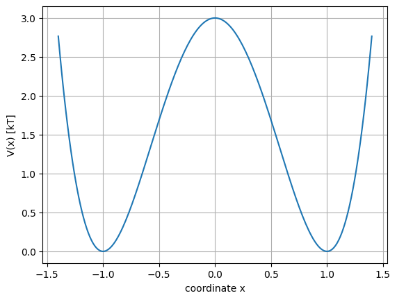
1.1 Dynamics: overdamped Langevin on a double well

We evolve a single coordinate x with overdamped Langevin dynamics:

• a deterministic drift given by a double-well force field,

• plus Gaussian noise with diffusion coefficient D.

We integrate for a small internal number of steps each time AIMMD requests a new MD frame. That gives a trajectory that qualitatively behaves like a coarse-grained MD simulation.

def toy_mdrun(ts, G: float = 3.0, dt: float = 1e-4, D: float = 1.0):
    """Propagate one MDAnalysis `Timestep` using overdamped Langevin dynamics.

    Parameters
    ----------
    ts
        MDAnalysis timestep. We read/write positions in-place.
    G
        Barrier height parameter for the double-well potential.
    dt
        Internal integration time step.
    D
        Diffusion coefficient controlling the noise amplitude.

    Notes
    -----
    - We treat positions as a scalar `x` stored in `ts.positions[0, 0]`.
    - The update is repeated `n_inner=100` times per emitted trajectory frame.
    """
    sqrt2Dt = np.sqrt(2 * D * dt)
    x = ts.positions

    # Inner integrator steps per emitted trajectory frame.
    for _ in range(100):
        # Force from V(x) = G (x^2 - 1)^2  ->  dV/dx = 4G x (x^2 - 1)
        f = G * 4 * x * (x**2 - 1)
        x = x - f * dt + sqrt2Dt * np.random.normal()

    ts.positions = x


# Visualize the potential energy surface (in kT units).
G = toy_mdrun.__defaults__[0]
pes = lambda x: G * (x**2 - 1) ** 2

xgrid = np.linspace(-1.4, 1.4, 200)
plt.plot(xgrid, pes(xgrid))
plt.xlabel("coordinate x")
plt.ylabel("V(x) [kT]")
plt.grid(True)
plt.show()

1.2 Metastable states

We define two end states and a reactive region:

• A: x < -0.7

• B: x > 0.7

• R: the intermediate region, where shooting starts and where transitions happen

AIMMD expects a function that maps a trajectory (iterable of timesteps) to a per-frame array of labels.

def states_function(trajectory):
    """Assign a discrete state label to each trajectory frame."""
    labels = []
    for ts in trajectory:
        x = ts.positions[0][0]
        if x < -0.7:
            labels.append("A")
        elif x > 0.7:
            labels.append("B")
        else:
            labels.append("R")
    return np.array(labels, dtype="<U1")

2. Build an initial path

AIMMD needs at least one initial trajectory (or “path”) that connects regions of phase space. For this toy model we simply sweep the coordinate from left to right and write it as an XTC.

This is not a physical trajectory; it is just a convenient starting point for training and for seeding the first shooting points.

# Build a 1-atom MDAnalysis Universe with an in-memory trajectory.
universe = mda.Universe.empty(1, trajectory=True)
atoms = universe.atoms
ts = universe.trajectory.ts

# Write a simple sweep trajectory to disk.
initial_xtc = PosixPath("initial.xtc")
with mda.coordinates.XTC.XTCWriter(str(initial_xtc), n_atoms=1) as writer:
    for x in np.arange(-1.4, 1.4, 0.01):
        ts.positions = x
        writer.write(atoms)

print("Wrote:", initial_xtc.resolve())

Wrote: /home/covino-shared/data/lichtinger/LigandAIMMD/new_aimmd/AIMMD/examples/data/data/data/1d_double_well/initial.xtc

3. Define a minimal committor model

In AIMMD the committor (or a monotonic surrogate) is typically approximated by a small network.

Here we create a tiny MLP in a separate network.py module and instantiate it there. This mirrors the recommended project layout: the notebook imports a ready-to-use model object.

Why write a module instead of defining the class inline?

• aimmd.Params is meant to be serializable/reproducible: having the model defined in a file makes it easier to reload exactly the same architecture later.

# Write a standalone module that defines the model *and* constructs an instance.
# The notebook will import `network` (the instance), not `Network` (the class).

network_py = PosixPath("network.py")
network_py.write_text(
    '''"""
Network used by AIMMD.

This module is written by the notebook so the model can be imported from a
standalone file (similar to how it would be done in a normal project).
"""

import torch
import torch.nn as nn


class Network(nn.Module):
    """Small MLP mapping a 1D input to a 1D output."""

    def __init__(self, n: int = 64):
        super().__init__()

        # Optional metadata container (unused by forward, but harmless to keep).
        self.call_kwargs = {}

        self.input = nn.Linear(1, n)
        self.layer = nn.Linear(n, n)
        self.activation = nn.ReLU()
        self.output = nn.Linear(n, 1)

        self.reset_parameters()

    def forward(self, x):
        # AIMMD may pass coordinates with shape (n_frames, 3). We only use the first component.
        x = self.activation(self.input(x[:, :1]))
        x = self.activation(self.layer(x))
        x = self.output(x)
        return x

    def reset_parameters(self):
        self.input.reset_parameters()
        self.layer.reset_parameters()
        self.output.reset_parameters()


# Ready-to-use model instance (import this from the notebook).
network = Network()
''',
    encoding="utf-8",
)

print("Wrote:", network_py.resolve())

# Import the instance created in the module.
from network import network

network

Wrote: /home/covino-shared/data/lichtinger/LigandAIMMD/new_aimmd/AIMMD/examples/data/data/data/1d_double_well/network.py

Network(
  (input): Linear(in_features=1, out_features=64, bias=True)
  (layer): Linear(in_features=64, out_features=64, bias=True)
  (activation): ReLU()
  (output): Linear(in_features=64, out_features=1, bias=True)
)

4. Create aimmd.Params

Params is the single source of truth for a run: it stores

• the state definition,

• how to launch dynamics (engine + engine kwargs),

• the committor model,

• I/O conventions (working folders, filenames),

• and the sampling/training hyperparameters.

In a typical project you would create a params.py file. For a tutorial it is convenient to build Params inline; AIMMD still writes a reproducible parameters file when a run is initialized.

params = aimmd.Params(
    # states and dynamics
    states_function=states_function,
    engine="toy",
    toy_mdrun=toy_mdrun,

    # committor model
    network=network,

    # initial data
    initial_paths="initial.xtc",

    # sampling setup
    chain_type="tps",
    selection_pool_size=1,
)

params

Written full params with descriptions to 'params.py'

Params params.py

4.1 Inspect the initial path object

params.initial_paths returns AIMMD Path objects. Each Path stores a list of trajectory segments plus cached derived data (states, descriptors, values) when computed.

print("Initial paths:", params.initial_paths)

path0 = params.initial_paths[0]
print("First initial path:", path0)
print("  states:", np.unique(path0.states))
print("  type:", path0.type)
print("  n_frames:", len(path0))

Initial paths: PathEnsemble with 1 paths
First initial path: Path with 143 frames
  states: ['A' 'B' 'R']
  type: ARBA
  n_frames: 143

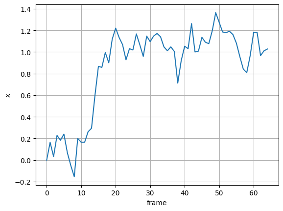
5. Sanity-check the engine

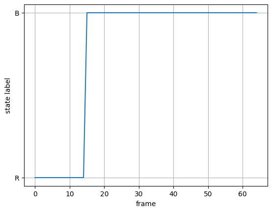
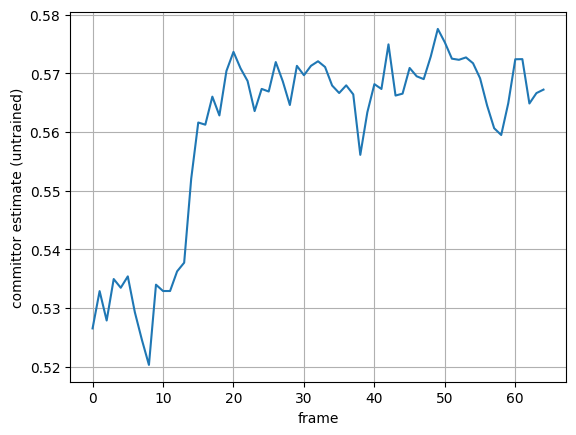
Before launching AIMMD, it is useful to check that:

• the engine can write a short trajectory,

• the state function behaves as expected,

• the committor model can be evaluated on coordinates.

This also illustrates how AIMMD uses a “simulation id” to name temporary outputs.

# Pick a starting frame from the middle of the sweep trajectory.
initial_path = params.initial_paths[0]
starting_frame = initial_path[len(initial_path) // 2]

# Run a short test simulation and write `test.xtc`.
params.initialize_simulation(starting_frame, "test")
params.run_simulation("test", walltime=1.0)

Warning: could not randomize velocities, set them to zero, please update params.topology
Appending to 'test.xtc'
[PID 2841654, TID 140357064955456: toy engine run] starting (Fri Mar  6 15:10:44 2026)
[PID 2841654, TID 140356981093952: toy engine check] starting (Fri Mar  6 15:10:44 2026)
[PID 2841654, TID 140357064955456: toy engine run] exited correctly
[PID 2841654, TID 140356981093952: toy engine check] exited correctly

test_path = aimmd.Path("test.xtc")

plt.plot(test_path.positions[:, 0, 0])
plt.xlabel("frame")
plt.ylabel("x")
plt.grid(True)
plt.show()

plt.figure()
plt.plot(params.states_function(test_path))
plt.xlabel("frame")
plt.ylabel("state label")
plt.grid(True)
plt.show()

# Evaluate the (untrained) network output -> expit() maps logits to (0, 1).
plt.figure()
plt.plot(expit(params.values_function(test_path.positions)))
plt.xlabel("frame")
plt.ylabel("committor estimate (untrained)")
plt.grid(True)
plt.show()

6. Launch an AIMMD run (run1)

aimmd.Launcher orchestrates:

• training rounds,

• one or more shooting chains (TPS or RFPS),

• optional free simulations,

• job-script creation for clusters.

The run is placed in a folder (run1/ here).

launcher = aimmd.Launcher(params, "run1")
launcher

Launcher of 1 run ('run1')

6.1 One training round only

Calling launcher.run(0) performs a single training round without launching shooting chains and without free simulations. This is the smallest useful run: it produces a trained model from whatever training data is available (initial path endpoints here).

launcher.run(0)

Assigned parameters file 'params.py'
+++ created 'run1'
+++ created 'run1/initialARB'
+++ saved 'run1/initialARB/initial.xtc.trr' (from: 'initial.xtc')
+++ saved 'run1/initialARB/initial.xtc.trr.states.npy'
[PID 2841654, TID 140364353083200: "run1" ARB trainer] starting (Fri Mar  6 15:11:18 2026)
...   args: ('params.py', 'run1', np.int64(0), np.int64(28), 1, 'stdout', inf, np.float64(inf), np.float64(inf), 59.0, 'train', np.float64(1.0), False)
Press Control+C to interrupt.

Worker's resources info
-----------------------
LocalID 0
CPU ids: 0,1,2,3,4,5,6,7,8,9,10,11,12,13,14,15,16,17,18,19,20,21,22,23,24,25,26,27
GPU ids: 0
-----------------------
run1: 0 trajs [00:00, ? trajs/s]
Loading pre-existing network parameters (Fri Mar  6 15:11:18 2026)
Warning: [Errno 2] No such file or directory: 'run1/networkARB.h5'

Loading current path ensemble (Fri Mar  6 15:11:18 2026)
... 0 new frames

Training the network (round 1, (Fri Mar  6 15:11:18 2026))

Collected         1 in A frames (     1 paths),
                  1 in B frames (     1 paths),
                  0 free A to A frames (     0 paths),
                  0 free B to B frames (     0 paths),
                  0 free A to B frames (     0 paths),
                  0 free B to A frames (     0 paths),
                  0 shot A to A frames (     0 paths),
                  0 shot B to B frames (     0 paths),
                  0 shot A to B frames (     0 paths), and
                  0 shot B to A frames (     0 paths)
   TOTAL:         2 frames

Calculating shooting results and sel. probabilities (Fri Mar  6 15:11:18 2026)

Bins [-inf  inf]

Disabling early stopping since total samples 2 < 1000 min samples.

Training set size 2
Transforming descriptors (Fri Mar  6 15:11:18 2026)
Resetting the network parameters (Fri Mar  6 15:11:18 2026)

Starting the training cycle (Fri Mar  6 15:11:18 2026)



























    loss 6.265e-01, scale 0.274, range (-0.024, 0.274)


























    loss 5.624e-01, scale 0.373, range (-0.204, 0.373)


























    loss 5.053e-01, scale 0.488, range (-0.366, 0.488)


























    loss 4.482e-01, scale 0.619, range (-0.536, 0.619)


























    loss 3.925e-01, scale 0.771, range (-0.708, 0.771)


























    loss 3.384e-01, scale 0.952, range (-0.882, 0.952)


























    loss 2.876e-01, scale 1.153, range (-1.063, 1.153)


























    loss 2.411e-01, scale 1.365, range (-1.255, 1.365)


























    loss 2.003e-01, scale 1.579, range (-1.454, 1.579)


























    loss 1.656e-01, scale 1.794, range (-1.652, 1.794)


























    loss 1.375e-01, scale 2.010, range (-1.841, 2.010)


























    loss 1.143e-01, scale 2.218, range (-2.027, 2.218)


























    loss 9.577e-02, scale 2.418, range (-2.207, 2.418)


























    loss 8.027e-02, scale 2.607, range (-2.381, 2.607)


























    loss 6.789e-02, scale 2.788, range (-2.543, 2.788)


























    loss 5.812e-02, scale 2.961, range (-2.696, 2.961)


























    loss 5.029e-02, scale 3.125, range (-2.840, 3.125)


























    loss 4.357e-02, scale 3.278, range (-2.978, 3.278)


























    loss 3.807e-02, scale 3.422, range (-3.111, 3.422)


























    loss 3.358e-02, scale 3.558, range (-3.237, 3.558)

501it [02:02,  4.08it/s]

Training took 123.0s
    501 epochs
    last loss 3.333e-02
    last scale 3.563
    last range (-3.242, 3.563)
*** training completed (Fri Mar  6 15:13:21 2026)

Loading current path ensemble (Fri Mar  6 15:13:21 2026)
... 0 new frames

Updating the values of all reactive R frames (Fri Mar  6 15:13:21 2026)
... computed 0 values

Obtaining the adaptation bins (Fri Mar  6 15:13:21 2026)
    bins: [  -inf -0.5   -0.375 -0.25  -0.125  0.     0.125  0.25   0.375  0.5
    inf]

Reweighting the full path ensemble (Fri Mar  6 15:13:21 2026)
    k12 estimate: nan [1/dt]
    k21 estimate: nan [1/dt]
    0 frames

Projecting the TPE density (Fri Mar  6 15:13:21 2026)
    densities: [0.1 0.1 0.1 0.1 0.1 0.1 0.1 0.1 0.1 0.1]

Substituting '...values.npy' files with '...new.npy' (Fri Mar  6 15:13:21 2026)

Saving network parameters to run1/networkARB.h5 (Fri Mar  6 15:13:21 2026)

Saving bins and densities (Fri Mar  6 15:13:21 2026)

Loading current path ensemble (Fri Mar  6 15:13:21 2026)
... 0 new frames
[PID 2841654, TID 140364353083200: "run1" ARB trainer] exited correctly

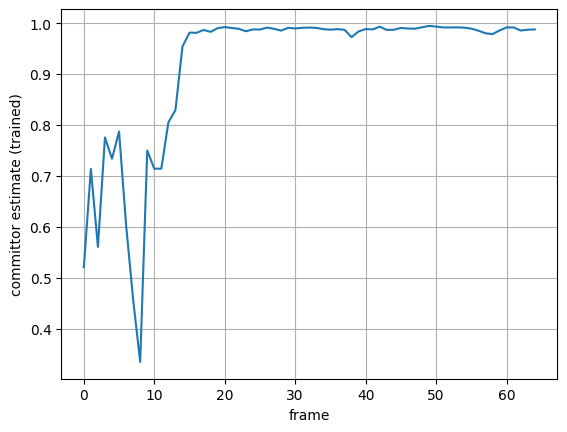
6.2 Load the trained network and evaluate committor predictions

The trained network weights are written into the run folder. Here we reload them into the in-memory model instance and re-evaluate the committor along the test trajectory.

plt.figure()

# Load the weights produced by the training round.
network.load_state_dict(torch.load("run1/networkARB.h5"))

# Re-evaluate on the test trajectory.
plt.plot(expit(params.values_function(test_path.positions)))
plt.xlabel("frame")
plt.ylabel("committor estimate (trained)")
plt.grid(True)
plt.show()

7. Run TPS shooting

A TPS chain repeatedly:

1. selects a shooting point from a selection pool,

2. launches short unbiased simulations forward/backward,

3. accepts or rejects the resulting path according to the ensemble definition.

In this tutorial we keep everything small (few steps, short walltime). On a terminal you will typically see a live progress bar; in notebooks output may appear line-by-line depending on the stdout backend.

# One TPS chain, limited number of shooting steps.
launcher.run(n=1, nsteps=30, walltime=120)

Assigned parameters file 'params.py'
--- removed run1/initialARB/initial.xtc.trr.states.npy
--- removed run1/initialARB/initial.xtc.trr
+++ saved 'run1/initialARB/initial.xtc.trr' (from: 'initial.xtc')
+++ saved 'run1/initialARB/initial.xtc.trr.states.npy'
+++ created run1/chainR0
[PID 2847995, TID 140546883319616: "run1" ARB trainer] starting (Fri Mar  6 15:13:47 2026)
...   args: ('params.py', 'run1', np.int64(1), np.int64(14), 1, 'trainARB.log', 120.0, np.float64(30.0), np.float64(inf), 59.0, 'train', np.float64(inf), True)
[PID 2847994, TID 140597403236160: "run1" chainR0] starting (Fri Mar  6 15:13:47 2026)
...   args: ('params.py', 'run1', np.int64(0), np.int64(14), 1, 'chainR0/worker.log', inf, inf, inf, 59.0, 'shoot', 'R', 0, False)
[PID 2847995, TID 140546883319616: "run1" ARB trainer] exited correctly
[PID 2847994, TID 140597403236160: "run1" chainR0] exited correctly

7.1 Append and expand to multiple chains in parallel

n=3 launches three independent shooting chains (separate workers), appending to the already simulated one (run1/shootR0). Here we stop the run after a cumulative number of produced frames across chains (nframes=10000).

launcher.run(n=3, nsteps=50, walltime=60)

Assigned parameters file 'params.py'
--- removed run1/initialARB/initial.xtc.trr.states.npy
--- removed run1/initialARB/initial.xtc.trr.values.npy
--- removed run1/initialARB/initial.xtc.trr
+++ saved 'run1/initialARB/initial.xtc.trr' (from: 'initial.xtc')
+++ saved 'run1/initialARB/initial.xtc.trr.states.npy'
[PID 2856590, TID 139817411200832: "run1" chainR2] starting (Fri Mar  6 15:23:11 2026)
...   args: ('params.py', 'run1', np.int64(2), np.int64(7), 1, 'chainR2/worker.log', inf, inf, inf, 59.0, 'shoot', 'R', 2, False)
[PID 2856588, TID 140093756548928: "run1" chainR0] starting (Fri Mar  6 15:23:11 2026)
...   args: ('params.py', 'run1', np.int64(0), np.int64(7), 1, 'chainR0/worker.log', inf, inf, inf, 59.0, 'shoot', 'R', 0, False)
[PID 2856591, TID 139928508892992: "run1" ARB trainer] starting (Fri Mar  6 15:23:11 2026)
...   args: ('params.py', 'run1', np.int64(3), np.int64(7), 1, 'trainARB.log', 60.0, np.float64(50.0), np.float64(inf), 59.0, 'train', np.float64(inf), True)
[PID 2856589, TID 140149688739648: "run1" chainR1] starting (Fri Mar  6 15:23:11 2026)
...   args: ('params.py', 'run1', np.int64(1), np.int64(7), 1, 'chainR1/worker.log', inf, inf, inf, 59.0, 'shoot', 'R', 1, False)
[PID 2856591, TID 139928508892992: "run1" ARB trainer] exited correctly
[PID 2856590, TID 139817411200832: "run1" chainR2] exited correctly
[PID 2856588, TID 140093756548928: "run1" chainR0] exited correctly
[PID 2856589, TID 140149688739648: "run1" chainR1] exited correctly

7.2 Simulate without retraining (optional)

If you want to keep the model fixed but still simulated and refresh selection densities/bins, you can run with nrounds=-1. This is mainly useful for analysis workflows.

launcher.run(n=3, walltime=60, nrounds=-1)

Assigned parameters file 'params.py'
--- removed run1/initialARB/initial.xtc.trr.states.npy
--- removed run1/initialARB/initial.xtc.trr.values.npy
--- removed run1/initialARB/initial.xtc.trr
+++ saved 'run1/initialARB/initial.xtc.trr' (from: 'initial.xtc')
+++ saved 'run1/initialARB/initial.xtc.trr.states.npy'
[PID 2858258, TID 140688390190912: "run1" ARB trainer] starting (Fri Mar  6 15:24:55 2026)
...   args: ('params.py', 'run1', np.int64(3), np.int64(7), 1, 'trainARB.log', 60.0, np.float64(inf), np.float64(inf), 59.0, 'train', np.float64(-1.0), True)
[PID 2858257, TID 140441812629312: "run1" chainR2] starting (Fri Mar  6 15:24:55 2026)
...   args: ('params.py', 'run1', np.int64(2), np.int64(7), 1, 'chainR2/worker.log', inf, inf, inf, 59.0, 'shoot', 'R', 2, False)
[PID 2858256, TID 140416463652672: "run1" chainR1] starting (Fri Mar  6 15:24:55 2026)
...   args: ('params.py', 'run1', np.int64(1), np.int64(7), 1, 'chainR1/worker.log', inf, inf, inf, 59.0, 'shoot', 'R', 1, False)
[PID 2858255, TID 139748750776128: "run1" chainR0] starting (Fri Mar  6 15:24:59 2026)
...   args: ('params.py', 'run1', np.int64(0), np.int64(7), 1, 'chainR0/worker.log', inf, inf, inf, 59.0, 'shoot', 'R', 0, False)
[PID 2858258, TID 140688390190912: "run1" ARB trainer] exited correctly
[PID 2858255, TID 139748750776128: "run1" chainR0] exited correctly
[PID 2858257, TID 140441812629312: "run1" chainR2] exited correctly
[PID 2858256, TID 140416463652672: "run1" chainR1] exited correctly

8. Cluster execution (SLURM job script template)

For real systems you will typically run AIMMD on a cluster. Launcher.create_job() writes a job script that starts the required worker processes.

Here we generate a small script for inspection.

launcher.create_job("job.sh", 2, 1, 1)
print(PosixPath("job.sh").read_text())

Assigned parameters file 'params.py'
--- removed run1/initialARB/initial.xtc.trr.states.npy
--- removed run1/initialARB/initial.xtc.trr
+++ saved 'run1/initialARB/initial.xtc.trr' (from: 'initial.xtc')
+++ saved 'run1/initialARB/initial.xtc.trr.states.npy'
+++ created run1/freeA
+++ created run1/freeB
#!/bin/bash -x
#SBATCH --job-name=AIMMD
#SBATCH --mail-type=FAIL
#SBATCH --ntasks-per-node=1
#SBATCH --cpus-per-task=1
#SBATCH --nodes=5
#SBATCH --time=24:00:00

# default names
PYTHON="/home/lichtinger/anaconda3/envs/new_aimmd/bin/python"
WORKER="/home/covino-shared/data/lichtinger/LigandAIMMD/new_aimmd/AIMMD/aimmd/worker/run.py"

# enable job control
set -m

# workers
# "run1" freeA (worker0)
srun --exclusive --nodes=1 --ntasks=1 --cpus-per-task=1 --gpus-per-task=0 \
  "${PYTHON}" "${WORKER}" "params.py" "run1" "0" "skip" "skip" "freeA/worker0.log" "inf" "inf" "inf" "59.0" "free" "A" "0" "1" "True" &

# "run1" freeB (worker0)
srun --exclusive --nodes=1 --ntasks=1 --cpus-per-task=1 --gpus-per-task=0 \
  "${PYTHON}" "${WORKER}" "params.py" "run1" "0" "skip" "skip" "freeB/worker0.log" "inf" "inf" "inf" "59.0" "free" "B" "0" "1" "True" &

# "run1" chainR0
srun --exclusive --nodes=1 --ntasks=1 --cpus-per-task=1 --gpus-per-task=0 \
  "${PYTHON}" "${WORKER}" "params.py" "run1" "0" "skip" "skip" "chainR0/worker.log" "inf" "inf" "inf" "59.0" "shoot" "R" "0" "" &

# "run1" chainR1
srun --exclusive --nodes=1 --ntasks=1 --cpus-per-task=1 --gpus-per-task=0 \
  "${PYTHON}" "${WORKER}" "params.py" "run1" "0" "skip" "skip" "chainR1/worker.log" "inf" "inf" "inf" "59.0" "shoot" "R" "1" "" &

# "run1" ARB trainer
srun --exclusive --nodes=1 --ntasks=1 --cpus-per-task=1 --gpus-per-task=0 \
  "${PYTHON}" "${WORKER}" "params.py" "run1" "0" "skip" "skip" "trainARB.log" "inf" "inf" "inf" "59.0" "train" "inf" "True" &

# wait until any process exits
wait -n
scancel ${SLURM_JOB_ID}
wait

9. Inspect and analyze the generated paths

AIMMD stores all sampled paths on disk. The analysis entry point is the PathEnsemble associated with a run folder.

pathensemble = params.pathensemble("run1")
pathensemble

PathEnsemble with 38 paths

9.1 Transition path ensemble (TPE)

are_transitions() selects paths that start in one end state and end in the other. The resulting subset carries the statistical weights produced by TPS.

tpe = pathensemble[pathensemble.are_transitions()]
tpe, tpe.fnames, tpe.weights

(PathEnsemble with 17 paths,
 array(['run1/chainR0/path000002.xtc', 'run1/chainR0/path000005.xtc',
        'run1/chainR0/path000009.xtc', 'run1/chainR0/path000010.xtc',
        'run1/chainR0/path000011.xtc', 'run1/chainR0/path000015.xtc',
        'run1/chainR0/path000018.xtc', 'run1/chainR0/path000020.xtc',
        'run1/chainR1/path000004.xtc', 'run1/chainR1/path000007.xtc',
        'run1/chainR1/path000008.xtc', 'run1/chainR2/path000001.xtc',
        'run1/chainR2/path000002.xtc', 'run1/chainR2/path000003.xtc',
        'run1/chainR2/path000007.xtc', 'run1/chainR2/path000008.xtc',
        'run1/chainR2/path000009.xtc'], dtype='<U27'),
 array([3., 4., 1., 8., 0., 0., 2., 1., 3., 3., 0., 1., 1., 4., 1., 1., 1.]))

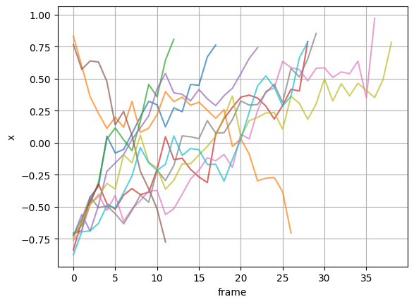
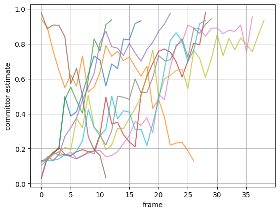
9.2 Visualize trajectories and committor traces

For the toy model the coordinate is just x(t) = positions[:, 0, 0]. We also plot the learned committor estimate along each path.

# Plot a handful of recent transition paths in coordinate space.
for path in tpe[-10:]:
    plt.plot(path.coordinates[:, 0], alpha=0.7)

plt.xlabel("frame")
plt.ylabel("x")
plt.grid(True)
plt.show()

# Plot committor estimates along the same paths.
for path in tpe[-10:]:
    path.compute(*params.compute_values_args)
    plt.plot(expit(path.values), alpha=0.7)

plt.xlabel("frame")
plt.ylabel("committor estimate")
plt.grid(True)
plt.show()

9.3 Forcing a recomputation of committor values (optional)

Normally the training process updates committor values consistently as the model changes. If you manually modify network weights and want to overwrite stored path.values, use overwrite=True.

params.update_network("run1")
pathensemble.compute(*params.compute_values_args, overwrite=True)

# You can also compute on subsets or single paths.
tpe.compute(*params.compute_values_args, overwrite=True)
_ = tpe[-1].compute(*params.compute_values_args, overwrite=True, return_result=True)

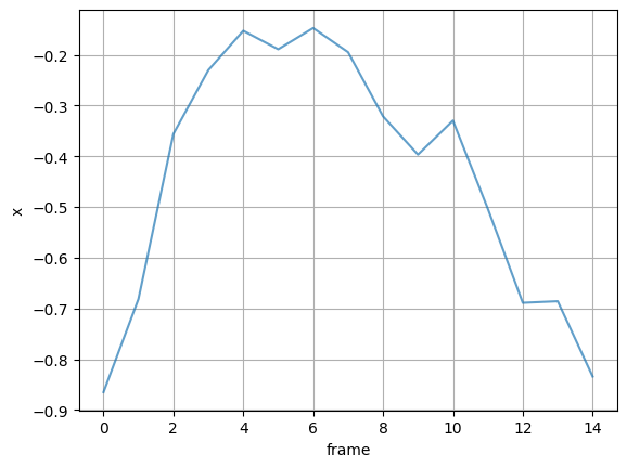
9.4 Other path types

Besides transition paths, the ensemble contains excursions such as ARA (leave A, enter R, return to A). extract() selects by path.type label.

for path in pathensemble.extract("ARA")[::10]:
    plt.plot(path.coordinates[:, 0], alpha=0.7)

plt.xlabel("frame")
plt.ylabel("x")
plt.grid(True)
plt.show()

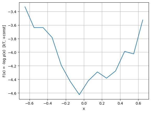
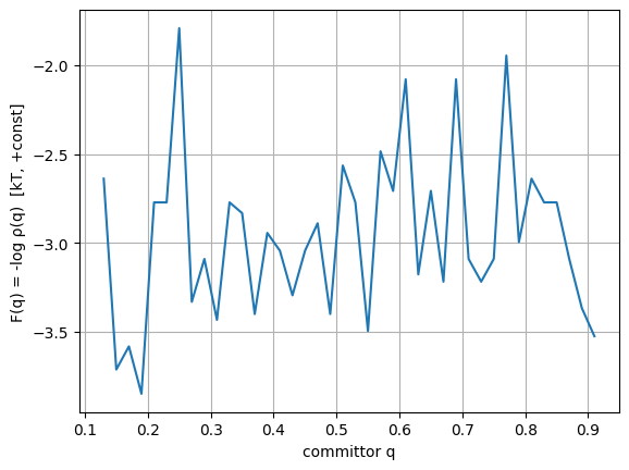
9.5 Simple projections: density and free energy along a coordinate

PathEnsemble.project() bins data extracted from each path and returns a normalized density estimate (up to the conventions of the underlying method).

Here we:

• project the TPE onto the coordinate x,

• and separately onto the committor values.

For a free-energy-like curve we plot F(x) = -log ρ(x) (up to an additive constant).

# Coordinate-space projection.
bins_x = np.arange(-1.4, 1.4, 0.1)
rho_x = tpe.project(bins=bins_x, function=lambda x: x[:, 0], source="coordinates")

x_centers = 0.5 * (bins_x[:-1] + bins_x[1:])
F_x = np.full_like(x_centers, np.nan, dtype=float)
mask = rho_x > 0
F_x[mask] = -np.log(rho_x[mask])

plt.plot(x_centers, F_x)
plt.grid(True)
plt.xlabel("x")
plt.ylabel("F(x) = -log ρ(x)  [kT, +const]")
plt.show()

# Committor-space projection.
# For this toy, committor values are stored as logits; apply expit() to map to (0, 1).
bins_q = np.linspace(0.0, 1.0, 51)

# Ensure values exist.
tpe.compute(*params.compute_values_args)

rho_q = tpe.project(bins=bins_q, function=lambda v: expit(v), source="values")
q_centers = 0.5 * (bins_q[:-1] + bins_q[1:])

F_q = np.full_like(q_centers, np.nan, dtype=float)
mask = rho_q > 0
F_q[mask] = -np.log(rho_q[mask])

plt.plot(q_centers, F_q)
plt.grid(True)
plt.xlabel("committor q")
plt.ylabel("F(q) = -log ρ(q)  [kT, +const]")
plt.show()

10. RFPS + free simulations (rate-oriented workflow)

RFPS (rejection-free path sampling) augments TPS by enhancing exploration within the reactive region, which can be helpful when you care about rates and need better coverage.

In this section we:

1. switch to RFPS and run a small production,

2. inspect the rate estimates reported in the training log,

3. reweight the produced path ensemble and project it.

# Switch to RFPS and increase the number of bins used internally for selection/reweighting.
params.chain_type = "rfps"
params.nbins = 10

# A larger selection pool can reduce the risk of repeatedly picking boundary-adjacent points.
# (Keep values small for the toy tutorial.)
# params.selection_pool_size = 10  # uncomment if desired

launcher = aimmd.Launcher(params, "run2")

# Run with multiple workers (arguments depend on your AIMMD version/configuration).
launcher.run(2, 2, 2, nsteps=50, walltime=120)

run1: 0 trajs [16:14, ? trajs/s]
run1: 0 frames [16:14, ? frames/s]
Written full params with descriptions to 'params1.py'
+++ created 'run2'
+++ created 'run2/initialARB'
+++ saved 'run2/initialARB/initial.xtc.trr' (from: 'initial.xtc')
+++ saved 'run2/initialARB/initial.xtc.trr.states.npy'
+++ created run2/freeA
+++ created run2/freeB
+++ created run2/chainR0
+++ created run2/chainR1
[PID 2860898, TID 140054408648512: "run2" freeA (worker1)] starting (Fri Mar  6 15:27:42 2026)
...   args: ('params1.py', 'run2', np.int64(1), np.int64(4), 1, 'freeA/worker1.log', inf, inf, inf, 59.0, 'free', 'A', 1, np.int64(2), np.True_)
[PID 2860904, TID 140001152579392: "run2" ARB trainer] starting (Fri Mar  6 15:27:42 2026)
...   args: ('params1.py', 'run2', np.int64(6), np.int64(4), 1, 'trainARB.log', 120.0, np.float64(50.0), np.float64(inf), 59.0, 'train', np.float64(inf), True)
[PID 2860897, TID 140179936343872: "run2" freeA (worker0)] starting (Fri Mar  6 15:27:42 2026)
[PID 2860903, TID 140126057084736: "run2" chainR1] starting (Fri Mar  6 15:27:42 2026)
...   args: ('params1.py', 'run2', np.int64(0), np.int64(4), 1, 'freeA/worker0.log', inf, inf, inf, 59.0, 'free', 'A', 0, np.int64(2), np.True_)
...   args: ('params1.py', 'run2', np.int64(5), np.int64(4), 1, 'chainR1/worker.log', inf, inf, inf, 59.0, 'shoot', 'R', 1, False)
[PID 2860901, TID 139914785236800: "run2" chainR0] starting (Fri Mar  6 15:27:42 2026)
...   args: ('params1.py', 'run2', np.int64(4), np.int64(4), 1, 'chainR0/worker.log', inf, inf, inf, 59.0, 'shoot', 'R', 0, False)
[PID 2860899, TID 140114694854464: "run2" freeB (worker0)] starting (Fri Mar  6 15:27:44 2026)
...   args: ('params1.py', 'run2', np.int64(2), np.int64(4), 1, 'freeB/worker0.log', inf, inf, inf, 59.0, 'free', 'B', 0, np.int64(2), np.True_)
[PID 2860900, TID 140063352399680: "run2" freeB (worker1)] starting (Fri Mar  6 15:27:44 2026)
...   args: ('params1.py', 'run2', np.int64(3), np.int64(4), 1, 'freeB/worker1.log', inf, inf, inf, 59.0, 'free', 'B', 1, np.int64(2), np.True_)
[PID 2860904, TID 140001152579392: "run2" ARB trainer] exited correctly
[PID 2860900, TID 140063352399680: "run2" freeB (worker1)] exited correctly
[PID 2860898, TID 140054408648512: "run2" freeA (worker1)] exited correctly
[PID 2860897, TID 140179936343872: "run2" freeA (worker0)] exited correctly
[PID 2860899, TID 140114694854464: "run2" freeB (worker0)] exited correctly
[PID 2860903, TID 140126057084736: "run2" chainR1] exited correctly
[PID 2860901, TID 139914785236800: "run2" chainR0] exited correctly

10.1 Load the RFPS ensemble and count transitions

pathensemble = params.pathensemble("run2")
print(pathensemble, pathensemble.are_transitions().sum(), "transitions")

PathEnsemble with 2015 paths 25 transitions

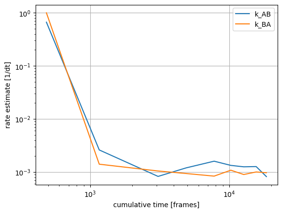
10.2 Rate estimates from the training log

The trainer periodically reports cumulative-time rate estimates. These become meaningful only after you have accumulated enough independent transitions (think: order 10–100 for stable estimates in real systems).

from aimmd.analysis.utils import extract_rate_estimates_from_log_file

t, k12, k21 = extract_rate_estimates_from_log_file("run2/trainARB.log")

plt.plot(t, k12, label="k_AB")
plt.plot(t, k21, label="k_BA")
plt.gca().set_yscale("log")
plt.gca().set_xscale("log")
plt.grid(True)
plt.xlabel("cumulative time [frames]")
plt.ylabel("rate estimate [1/dt]")
plt.legend()
plt.show()

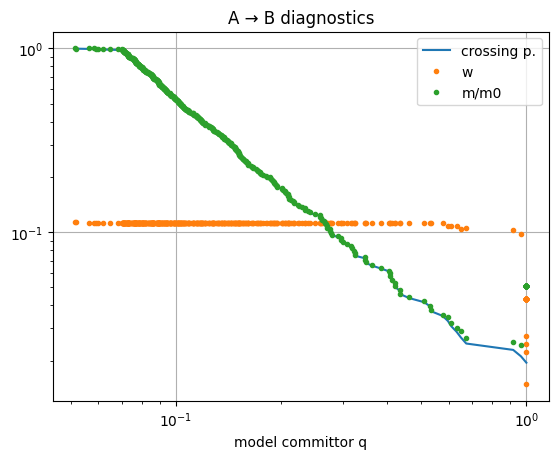
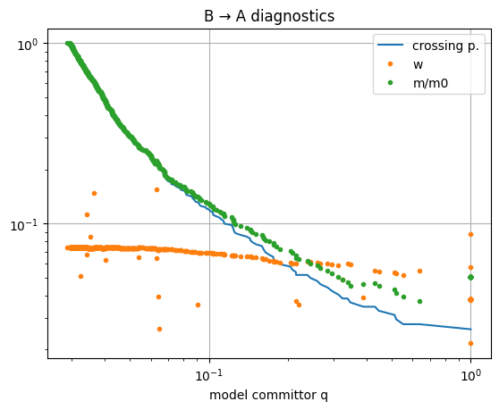
10.3 Reweight and compute crossing-probability diagnostics

For RFPS workflows it is often helpful to:

• recompute committor values for all frames (including state interiors),

• run reweighting for both directions,

• inspect crossing probabilities vs committor.

The PathEnsemble.reweight() helper returns several intermediate arrays used for diagnostics.

params.update_network("run2")

# Ensure committor values exist for all frames.
n_new_values = pathensemble.compute(*params.compute_values_args)
print("computed", n_new_values, "new values")

rw_p = params.reweight_parameters.copy()

# Reweight both directions.
result_AB = pathensemble.reweight(params.states, **rw_p)
result_BA = pathensemble.reweight(params.states[::-1], **rw_p)

w1, i1, factors1, shooting_values1, extremes1, xP1, f1, m1 = result_AB
w2, i2, factors2, shooting_values2, extremes2, xP2, f2, m2 = result_BA

computed 2608 new values

# Crossing probability diagnostics.
plt.plot(expit(extremes1), xP1, label="crossing p.")
plt.plot(expit(extremes1), w1[i1], ".", label="w")
plt.plot(expit(extremes1), m1 / m1[0], ".", label="m/m0")
plt.gca().set_xscale("log")
plt.gca().set_yscale("log")
plt.grid(True)
plt.title("A → B diagnostics")
plt.xlabel("model committor q")
plt.legend()
plt.show()

plt.figure()
plt.plot(expit(extremes2), xP2, label="crossing p.")
plt.plot(expit(extremes2), w2[i2], ".", label="w")
plt.plot(expit(extremes2), m2 / m2[0], ".", label="m/m0")
plt.gca().set_xscale("log")
plt.gca().set_yscale("log")
plt.grid(True)
plt.title("B → A diagnostics")
plt.xlabel("model committor q")
plt.legend()
plt.show()

# Simple rate-from-mean-length diagnostic (toy-level; do not over-interpret).
lengths = pathensemble.n_frames.astype(float)

k12_est = np.sum(w1 * lengths)
k12_est = 1.0 / k12_est if k12_est else np.nan

k21_est = np.sum(w2 * lengths)
k21_est = 1.0 / k21_est if k21_est else np.nan

print(f"k_AB estimate: {k12_est:.3e} [1/dt]")
print(f"k_BA estimate: {k21_est:.3e} [1/dt]")
print(f"total frames: {pathensemble.n_frames.sum()}")

k_AB estimate: 8.930e-04 [1/dt]
k_BA estimate: 1.283e-03 [1/dt]
total frames: 23584

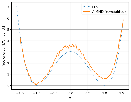
10.4 Project the (reweighted) ensemble

For a quick qualitative check we combine weights from both directions and compare:

• the true potential energy surface V(x) (known analytically),

• a free-energy-like curve from the projected reweighted ensemble.

# Combine weights for a simple "overall" projection.
pathensemble.weights = w1 + w2

coords = np.concatenate(pathensemble.coordinates)[:, 0]
bins = np.linspace(coords.min(), coords.max(), 101)
rho = pathensemble.project(bins=bins, function=lambda x: x[:, 0], source="coordinates")

x_centers = 0.5 * (bins[:-1] + bins[1:])
F = np.full_like(x_centers, np.nan, dtype=float)
mask = rho > 0
F[mask] = -np.log(rho[mask])
F = F - np.nanmin(F)

plt.plot(x_centers, pes(x_centers), ":", label="PES")
plt.plot(x_centers, F, label="AIMMD (reweighted)")
plt.grid(True)
plt.legend()
plt.xlabel("x")
plt.ylabel("free energy [kT, +const]")
plt.show()

# Free energy in logit-committor space.
values = np.concatenate(pathensemble.values)
bins = np.linspace(values.min(), values.max(), 101)
rho = pathensemble.project(bins=bins)  # default source='values'
x_centers = 0.5 * (bins[:-1] + bins[1:])

F = np.full_like(x_centers, np.nan, dtype=float)
mask = rho > 0
F[mask] = -np.log(rho[mask])

plt.plot(x_centers, F)
plt.grid(True)
plt.xlabel("logit committor")
plt.ylabel("F [kT, +const]")
plt.show()

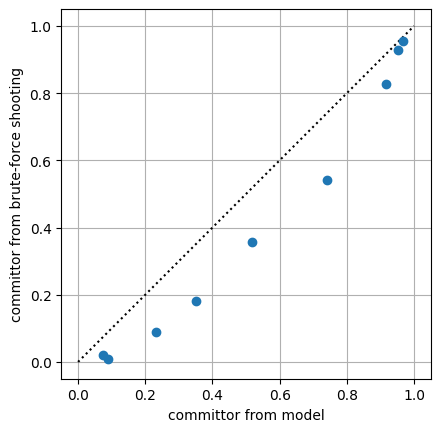
11. Committor validation by brute-force shooting (optional)

A pragmatic way to validate a learned committor is to:

1. sample configurations across committor bins,

2. launch many short unbiased shootings from each configuration,

3. estimate the empirical committor as the fraction of shootings that reach B before A,

4. compare empirical committor vs model prediction.

This is expensive for real systems, but cheap for the toy model.

# Sample configurations approximately uniformly across logit-committor bins.
bins = np.linspace(-4, 4, 11)
print("committor bin boundaries:", expit(bins))

validation_set = aimmd.Path()
excursions = pathensemble[pathensemble.are_excursions()]

for vmin, vmax in zip(bins[:-1], bins[1:]):
    validation_set += excursions.sample(1, vmin=vmin, vmax=vmax)

validation_set.write("committor_validation.xtc", overwrite=True)
validation_set.values

committor bin boundaries: [0.018 0.039 0.083 0.168 0.31  0.5   0.69  0.832 0.917 0.961 0.982]

array([-2.542, -2.336, -1.198, -0.62 ,  0.069,  1.051,  2.379,  2.983,
        3.353], dtype=float32)

# Reuse the validation set as the initial path list.
params.initial_paths = "committor_validation.xtc"

# Run brute-force shooting in "sweep" mode (no training).
launcher = aimmd.Launcher(params, "validation")

nframes = len(aimmd.Path("committor_validation.xtc"))
launcher.run(5, reactive_region_mode="sweep", nsteps=10 * nframes)

Warning: the initial trajectory 'committor_validation.xtc' has no 'ARB' transitions (path types: RRR), taking it as it is.
Perhaps you are using it for brute-force shooting?
Written full params with descriptions to 'params2.py'
+++ created 'validation'
+++ created 'validation/initialARB'
+++ saved 'validation/initialARB/committor_validation.xtc.trr' (from: 'committor_validation.xtc')
+++ saved 'validation/initialARB/committor_validation.xtc.trr.states.npy'
+++ created validation/sweepR0
+++ created validation/sweepR1
+++ created validation/sweepR2
+++ created validation/sweepR3
+++ created validation/sweepR4

[PID 2864260, TID 140451579459392: "validation" sweepR2] starting (Fri Mar  6 15:31:02 2026)[PID 2864261, TID 140421569521472: "validation" sweepR3] starting (Fri Mar  6 15:31:02 2026)

...   args: ('params2.py', 'validation', np.int64(3), np.int64(5), 1, 'sweepR3/worker.log', inf, np.float64(90.0), np.float64(inf), 59.0, 'shoot', 'R', 3, True)...   args: ('params2.py', 'validation', np.int64(2), np.int64(5), 1, 'sweepR2/worker.log', inf, np.float64(90.0), np.float64(inf), 59.0, 'shoot', 'R', 2, True)

[PID 2864262, TID 140277611865920: "validation" sweepR4] starting (Fri Mar  6 15:31:02 2026)
...   args: ('params2.py', 'validation', np.int64(4), np.int64(5), 1, 'sweepR4/worker.log', inf, np.float64(90.0), np.float64(inf), 59.0, 'shoot', 'R', 4, True)
[PID 2864258, TID 140186524489536: "validation" sweepR0] starting (Fri Mar  6 15:31:02 2026)
...   args: ('params2.py', 'validation', np.int64(0), np.int64(5), 1, 'sweepR0/worker.log', inf, np.float64(90.0), np.float64(inf), 59.0, 'shoot', 'R', 0, True)
[PID 2864259, TID 140422497507136: "validation" sweepR1] starting (Fri Mar  6 15:31:02 2026)
...   args: ('params2.py', 'validation', np.int64(1), np.int64(5), 1, 'sweepR1/worker.log', inf, np.float64(90.0), np.float64(inf), 59.0, 'shoot', 'R', 1, True)
[PID 2864262, TID 140277611865920: "validation" sweepR4] exited correctly
[PID 2864260, TID 140451579459392: "validation" sweepR2] exited correctly
[PID 2864261, TID 140421569521472: "validation" sweepR3] exited correctly
[PID 2864258, TID 140186524489536: "validation" sweepR0] exited correctly
[PID 2864259, TID 140422497507136: "validation" sweepR1] exited correctly

# Compare model committor vs brute-force estimate.
validation_set = aimmd.Path("committor_validation.xtc")

x_model = expit(
    validation_set.compute(
        params.values_function,
        "",
        *params.compute_values_args[2:],
        return_result=True,
    )
)
x_model[:5], len(x_model)

(array([0.073, 0.088, 0.232, 0.35 , 0.517], dtype=float32), 9)

r = np.zeros((len(validation_set), 2), dtype=float)

for shot_paths in params.shot_paths("validation", "sweep"):
    r += shot_paths.shooting_results(sweep_size=len(validation_set))

y_empirical = r[:, 1] / (r[:, 0] + r[:, 1])

plt.plot([0, 1], [0, 1], ":", color="black")
plt.plot(x_model, y_empirical, "o")
plt.xlabel("committor from model")
plt.ylabel("committor from brute-force shooting")
plt.gca().set_aspect("equal", adjustable="box")
plt.grid(True)
plt.show()

12. Advanced: multistate periodic toy model (optional)

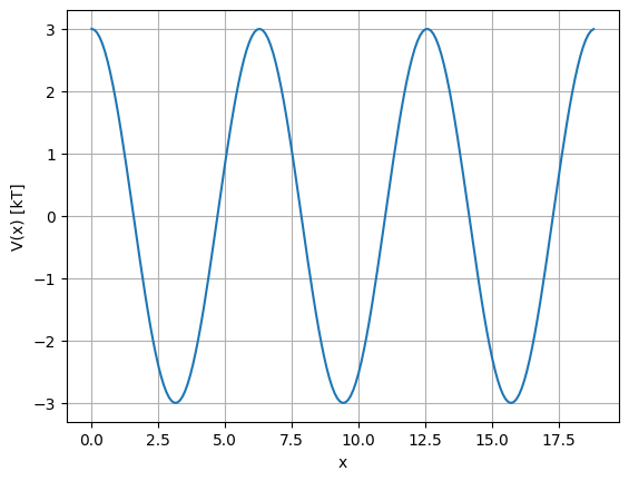
This final section demonstrates how to combine two AIMMD simulations that share the same engine but sample different portions of a periodic free-energy landscape.

We define 5 discrete regions along a periodic coordinate:

A — R — B — S — C

and build two coupled AIMMD setups:

• params1 for transitions between A ↔ B through R (ARB, BRA),

• params2 for transitions between B ↔ C through S (BSC, CSB).

This pattern generalizes to larger state networks in real applications.

# Switch to the periodic toy folder.
PERIODIC_DIR = PosixPath("../../data/1d_periodic").resolve()
PERIODIC_DIR.mkdir(parents=True, exist_ok=True)
os.chdir(PERIODIC_DIR)

print("Working directory:", os.getcwd())

# Copy the network module so imports still work from this folder.
os.system("cp ../1d_double_well/network.py .")

Working directory: /home/covino-shared/data/lichtinger/LigandAIMMD/new_aimmd/AIMMD/examples/data/data/data/1d_periodic

0

12.1 Periodic toy dynamics and state labeling

def toy_mdrun(ts, G: float = 3.0, dt: float = 1e-4, D: float = 10.0):
    """Overdamped Langevin on a periodic cosine potential."""
    sqrt2Dt = np.sqrt(2 * D * dt)
    x = ts.positions
    for _ in range(100):
        f = -G * np.sin(x)
        x = x - f * dt + sqrt2Dt * np.random.normal()
    ts.positions = x


def states_function(trajectory):
    """Partition x into five regions A/R/B/S/C along [0, 6π)."""
    labels = []
    for ts in trajectory:
        x = ts.positions[0][0]
        if x < np.pi + np.pi / 4:
            labels.append("A")
        elif x < 3 * np.pi - np.pi / 4:
            labels.append("R")
        elif x < 3 * np.pi + np.pi / 4:
            labels.append("B")
        elif x < 5 * np.pi - np.pi / 4:
            labels.append("S")
        else:
            labels.append("C")
    return np.array(labels, dtype="<U1")

# Initial path: sweep from 0 to 6π.
universe = mda.Universe.empty(1, trajectory=True)
atoms = universe.atoms
ts = universe.trajectory.ts

with mda.coordinates.XTC.XTCWriter("initial_cos.xtc", 1) as writer:
    for x in np.arange(0, np.pi * 6, 0.1):
        ts.positions = x
        writer.write(atoms)

# Visualize the periodic potential.
G = toy_mdrun.__defaults__[0]
pes = lambda x: G * np.cos(x)

xgrid = np.arange(0, np.pi * 6, 0.1)
plt.plot(xgrid, pes(xgrid))
plt.grid(True)
plt.xlabel("x")
plt.ylabel("V(x) [kT]")
plt.show()

12.2 Two coupled AIMMD setups

We create two independent Params objects. Each one uses a different descriptor transform that “recenters” the relevant reactive region near zero (useful for learning/stability).

from network import network

params1 = aimmd.Params(
    states_function=states_function,
    engine="toy",
    toy_mdrun=toy_mdrun,
    network=network,
    initial_paths="initial_cos.xtc",
)

# Center reactive region R near 0 (roughly around 2π).
def descriptor_transform(x):
    return x - np.pi * 2 
params1.descriptor_transform = descriptor_transform

params2 = aimmd.Params(
    states_function=states_function,
    engine="toy",
    toy_mdrun=toy_mdrun,
    states="BSC",
    network=network,
    initial_paths="initial_cos.xtc",
)

# Center reactive region S near 0 (roughly around 4π).
def descriptor_transform(x):
    return x - np.pi * 4
params2.descriptor_transform = descriptor_transform

launcher = aimmd.Launcher([params1, params2], "multistate")
launcher

Written full params with descriptions to 'params.py'

Written full params with descriptions to 'params1.py'

Launcher of 2 runs ('multistate', 'multistate')

# Example: you could dedicate one worker to free simulations in B (left as a comment).
launcher.run(n=1, n1=[1, 0], n2=[0, 1], walltime=100, nsteps=30)

Written full params with descriptions to 'params2.py'
+++ created 'multistate'
+++ created 'multistate/initialARB'
+++ saved 'multistate/initialARB/initial_cos.xtc.trr' (from: 'initial_cos.xtc')
+++ saved 'multistate/initialARB/initial_cos.xtc.trr.states.npy'
+++ created multistate/freeA
+++ created multistate/chainR0
Written full params with descriptions to 'params3.py'
+++ created 'multistate/initialBSC'
+++ saved 'multistate/initialBSC/initial_cos.xtc.trr' (from: 'initial_cos.xtc')
+++ saved 'multistate/initialBSC/initial_cos.xtc.trr.states.npy'
+++ created multistate/freeC
+++ created multistate/chainS0
[PID 2896728, TID 140301933188928: "multistate" ARB trainer] starting (Fri Mar  6 16:04:59 2026)[PID 2896727, TID 140381153994560: "multistate" chainR0] starting (Fri Mar  6 16:04:59 2026)[PID 2896731, TID 140185800263488: "multistate" chainS0] starting (Fri Mar  6 16:04:59 2026)


...   args: ('params3.py', 'multistate', np.int64(4), np.int64(4), 1, 'chainS0/worker.log', inf, inf, inf, 59.0, 'shoot', 'S', 0, False)...   args: ('params2.py', 'multistate', np.int64(1), np.int64(4), 1, 'chainR0/worker.log', inf, inf, inf, 59.0, 'shoot', 'R', 0, False)

...   args: ('params2.py', 'multistate', np.int64(2), np.int64(4), 1, 'trainARB.log', 100.0, np.float64(30.0), np.float64(inf), 59.0, 'train', np.float64(inf), True)
[PID 2896726, TID 140102015604544: "multistate" freeA (worker0)] starting (Fri Mar  6 16:04:59 2026)
...   args: ('params2.py', 'multistate', np.int64(0), np.int64(4), 1, 'freeA/worker0.log', inf, inf, inf, 59.0, 'free', 'A', 0, np.int64(1), np.True_)
[PID 2896732, TID 140328338749248: "multistate" BSC trainer] starting (Fri Mar  6 16:04:59 2026)
...   args: ('params3.py', 'multistate', np.int64(5), np.int64(4), 1, 'trainBSC.log', 100.0, np.float64(30.0), np.float64(inf), 59.0, 'train', np.float64(inf), True)
[PID 2896730, TID 140452535052096: "multistate" freeC (worker0)] starting (Fri Mar  6 16:05:02 2026)
...   args: ('params3.py', 'multistate', np.int64(3), np.int64(4), 1, 'freeC/worker0.log', inf, inf, inf, 59.0, 'free', 'C', 0, np.int64(1), np.True_)
[PID 2896728, TID 140301933188928: "multistate" ARB trainer] exited correctly
[PID 2896732, TID 140328338749248: "multistate" BSC trainer] exited correctly
[PID 2896730, TID 140452535052096: "multistate" freeC (worker0)] exited correctly
[PID 2896727, TID 140381153994560: "multistate" chainR0] exited correctly
[PID 2896726, TID 140102015604544: "multistate" freeA (worker0)] exited correctly
[PID 2896731, TID 140185800263488: "multistate" chainS0] exited correctly

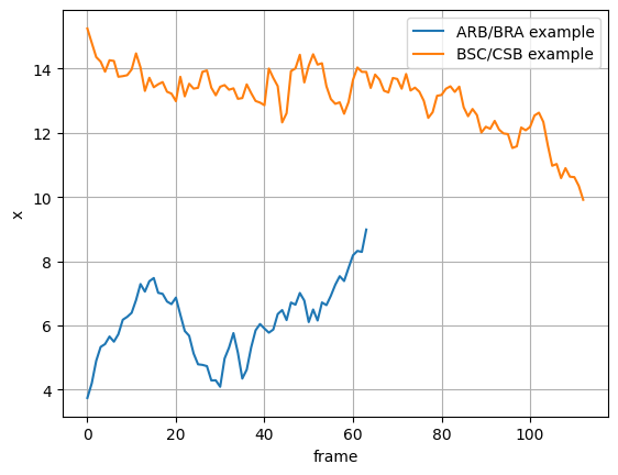
# Loading portions and inspecting them separately.
pathensemble1 = params1.pathensemble("multistate")  # ARB/BRA portion
pathensemble2 = params2.pathensemble("multistate")  # BSC/CSB portion

path1 = pathensemble1.extract("ARB", "BRA")[-1]
path2 = pathensemble2.extract("BSC", "CSB")[-1]

plt.plot(path1.coordinates[:, 0], label="ARB/BRA example")
plt.plot(path2.coordinates[:, 0], label="BSC/CSB example")
plt.legend()
plt.grid(True)
plt.xlabel("frame")
plt.ylabel("x")
plt.show()

12.3 Note on shared network instances

In this toy example, params1 and params2 share the same Python network object. That is convenient, but it means you must be explicit about which weights you load before computing values.

For independent training processes in real workflows, prefer separate model instances.

# If you want to overwrite committor values for one portion, reload the matching weights first.
params1.update_network("multistate")  # loads networkARB.h5 (depending on state naming)
pathensemble1.compute(*params1.compute_values_args, overwrite=True)

5150

12.4 Inspect the committor model for different transition portions

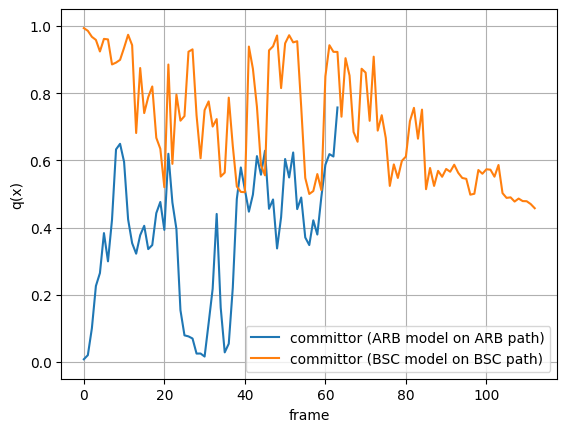
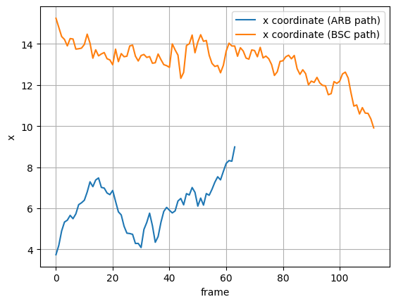
In the multistate periodic toy, we trained separate committor models for different reactive regions (e.g. ARB vs BSC). Even if the underlying coordinate x lives in different ranges (different periodic sectors), each model should output a consistent committor-like signal for its own transition region.

Important detail in this tutorial setup: params1 and params2 share the same Python network instance. Therefore, you must reload the right weights before computing committor values for each portion, otherwise you will silently evaluate with the wrong model.

# Pick one representative transition-like path from each portion.
# (Change the selectors if you want different types.)
path1 = pathensemble1.extract("ARB", "BRA")[-1]
path2 = pathensemble2.extract("BSC", "CSB")[-1]

# Because params1/params2 share the same `network` object, always reload weights
# before computing values for each portion.
params1.update_network("multistate")  # typically loads networkARB.h5
path1.compute(*params1.compute_values_args, overwrite=True)

params2.update_network("multistate")  # typically loads networkBSC.h5
path2.compute(*params2.compute_values_args, overwrite=True)

# `path.values` are usually logits (pre-sigmoid). Convert to committor in [0, 1].
q1 = path1.values
q2 = path2.values
p1 = expit(path1.values)
p2 = expit(path2.values)

plt.figure()
plt.plot(p1, label="committor (ARB model on ARB path)")
plt.plot(p2, label="committor (BSC model on BSC path)")
plt.xlabel("frame")
plt.ylabel("q(x)")
plt.ylim(-0.05, 1.05)
plt.grid(True)
plt.legend()

plt.figure()
plt.plot(path1.coordinates[:, 0], label="x coordinate (ARB path)")
plt.plot(path2.coordinates[:, 0], label="x coordinate (BSC path)")
plt.xlabel("frame")
plt.ylabel("x")
plt.grid(True)
plt.legend()

print("ARB path:   p min/max =", float(q1.min()), float(q1.max()))
print("BSC path:   p min/max =", float(q2.min()), float(q2.max()))

ARB path:   p min/max = -4.8349385261535645 1.1376829147338867
BSC path:   p min/max = -0.1708049327135086 5.035522937774658

13. Takeaways

• The toy engine + state function are the minimal pieces needed to run AIMMD.

• Params captures run configuration; Launcher executes sampling/training; PathEnsemble is the analysis entry point.

• In notebooks, multiprocessing output may be less polished than in terminals; logs in the run folder are the authoritative record.

From here, you can replace the toy engine with a real MD engine backend and replace the state function with physically meaningful order parameters (distances, contacts, RMSD, etc.).